A Brief History of RAID
Before modern storage arrays and cloud drives became everyday tools, enterprises faced a fundamental challenge: how to store growing volumes of data reliably and cost-effectively?
Storage systems had to keep pace with rapidly advancing processors and increasingly demanding business applications, but they were struggling.
By the mid-1980s, every serious data center still depended on the Single Large Expensive Drive (SLED).
- IBM’s flagship 3380 cabinet held approximately 2.52 GB data, sustained 3 MB/s transfer speed, averaged 16 ms seek time, and cost $81000–$142000—plus a cubic meter of floor space and a kilowatt of power.
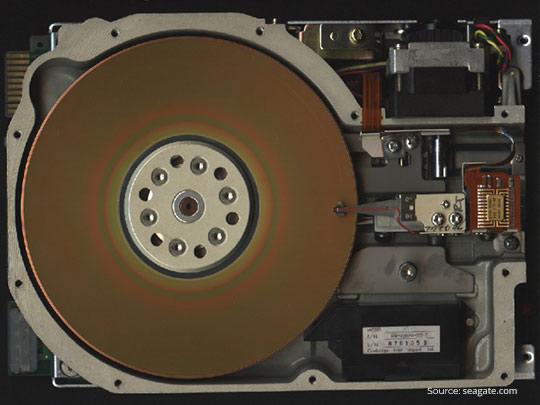
- Smaller computers fared no better: the first PC hard drive, the 5.25-inch ST-506 by Shugart Technology (now Seagate), had a capacity of just 5 MB and was priced at $1,500—a steep $300 per MB.
At the same time, Moore’s law remained largely true for CPUs and ever-cheaper DRAM, which doubled in speed or capacity every 18–24 months. This meant that transaction processing, SQL databases, and emerging client-server apps were issuing far more tiny random I/Os than any single spindle could serve.
Researchers from UC-Berkeley—David Patterson, Garth Gibson, and Randy Katz—quantified the gap: processor performance was climbing at 40% per year, yet a top-end disk’s mechanical latency was improving by barely 7% per year.
The result was what they called the looming “I/O crisis”—CPUs stalled, batch windows blew out, and enterprises were forced to stripe critical tables across hundreds of SLEDs.
This quick-and-dirty fix created new headaches.
- Cost ballooned linearly with each added SLED.
- Availability actually fell because more spindles meant more points of failure.
- Operators fought a losing battle against heat, power draw, and floor-space limits.
What the industry urgently needed was mainframe-class throughput and capacity, but at PC-class prices—without sacrificing reliability.
Those are exactly the constraints that inspired the storage-research community in the 1980s.
RAID: Origin and Definition
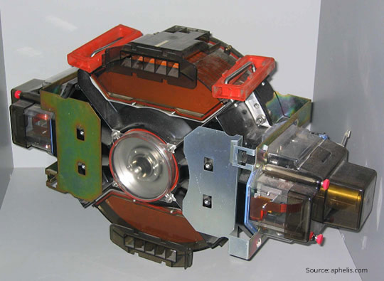
In late 1987, Patterson, Gibson, & Katz set a folding table in a UC-Berkeley lab with ten 100 MB Conner CP-3100 PC drives wired to an off-the-shelf SCSI controller.
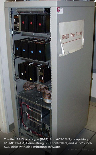
They were chasing one question: Could a pack of cheap PC disks outrun the reigning mainframe workhorse, the IBM 3380?
Their SIGMOD ‘88 paper, “A Case for Redundant Arrays of Inexpensive Disks (RAID),” supplied the hard numbers.
| Drive (1987) | Capacity | Transfer rate | Price/MB | Power | Volume |
| IBM 3380 AK4 | 7500 MB | ≈ 3 MB/s | $18–$10 | 6.6 kW | 24 ft³ |
| Fujitsu “Super Eagle” | 600 MB | ≈ 2.5 MB/s | $20–$17 | 640 W | 3.4 ft³ |
| Conner CP-3100 | 1000 MB | ≈ 1 MB/s | $11–$7 | 10 W | 0.03 ft³ |
They then modeled a Level 5 RAID built from 100 of those Conner drives (10 data + 2 parity per group).
The result:
- Approximately five times the I/O throughput, power, and floor-space efficiency of the IBM 3380
- Costing two orders of magnitude less per gigabyte
- Increasing calculated reliability, thanks to parity and hot-spare rebuilds
Put differently, an $11,000 array matched—and often exceeded—the $100,000 SLED on every metric that mattered.
That tabletop demo transformed RAID from idea to inevitability and kicked off the era of array engineering.
What the Name “Redundant Array of Independent Disks” Signifies
| Word | Why it matters |
| Redundant | Extra information (full copies or parity codes) is stored so the logical data stays online after a drive failure. |
| Array | Many physical drives are virtualized into one logical address space; the controller maps host block numbers to drive/sector locations, schedules I/O, and orchestrates rebuilds. |
| Independent (originally “Inexpensive”) | Commodity disks fail independently and cost far less per GB than a monolithic SLED. The RAID controller absorbs that higher failure rate to deliver a higher system MTTDL (Mean Time to Data Loss). |
| Disks | The scheme was born on spinning HDDs, but the math applies equally to SSDs and other drives. |
A RAID set is therefore a single virtual disk presented to the host, built from a group of cheap, failure-prone drives, having enough redundancy logic to guarantee data survival and to present higher aggregate performance.
Before we unpack specific RAID levels, we need three technical building blocks—striping, mirroring, and parity—and a few baseline terms.
- I/O (Input/Output): Every read or write request the host issues.
- Host: The server or controller that sends block requests over SAS, SATA, NVMe, or FC.
- Block (sector): The atomic unit (512 B–4 KiB) by which disks store and RAID algorithms calculate parity.
With that vocabulary in place, we can dive into how striping accelerates I/O, how mirroring gives instant redundancy, and how parity lets us rebuild lost data with elegant XOR math.
The Three Building Blocks of RAID—Striping, Mirroring, & Parity
Striping (Performance & Scale)
Striping is a technique that spreads data across multiple drives, allowing the drives to work in parallel. All the read-write heads operate simultaneously on corresponding platters, meaning more data can be processed in a shorter time. This dramatically increases performance compared to relying on a single disk.
The diagram below shows how striping works in a set of W drives. A strip is N contiguous blocks on one drive; a stripe is the set of aligned strips that spans W drives (the stripe width).
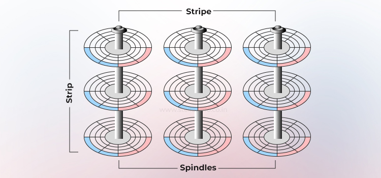
Stripe size = strip size × stripe width.
Choosing strip size is purely a matter of workload tuning. It can be small (16–64 KiB) for OLTP (online transaction processing) or large (256 KiB–1 MiB) for video streams.
By servicing each I/O request with several disks in parallel, sequential bandwidth scales almost linearly with W until the controller or bus saturates.
The RAID configuration with pure striping (i.e., no mirroring) is RAID 0, which doesn’t offer any redundancy—lose one member, lose the array!
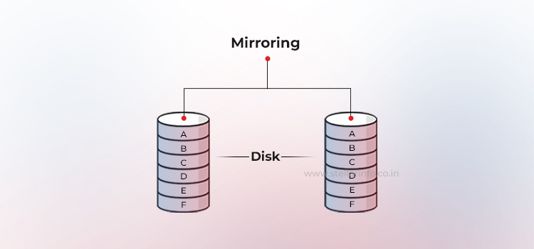
Mirroring (Instant Redundancy)
Mirroring is a technique where the same data is stored on two different disk drives. If one disk drive fails, the data remains fully intact on the surviving disk. The controller continues to service the host’s data requests from the healthy member of the mirrored pair, without interruption.
When the failed disk is replaced with a new one, the controller automatically copies the data from the surviving disk to the new disk—a process that is transparent to the host.
In a RAID configuration with mirroring (RAID 1), every write is dispatched to at least two drives. This creates duplicate data sets called sub-mirrors. The controller can satisfy reads from whichever sub-mirror is the least busy.
Enterprise operating systems and HBAs (Host Bus Adapters) even offer round-robin or geometric read policies to balance the load and trim seek time.
In mirroring, although write commands have to pay a small latency penalty (they must commit twice) and capacity efficiency is 50%, the benefits outweigh this: In case of drive failure, rebuilding is trivial—a straight copy from the surviving member to a spare.
Parity (Math-Based Redundancy)
Parity is a method to protect striped data from disk failure without the full cost of mirroring. Instead of duplicating all data, RAID arrays use an extra disk (or distributed space) to store parity—a mathematical summary of the data that allows the system to reconstruct lost information.
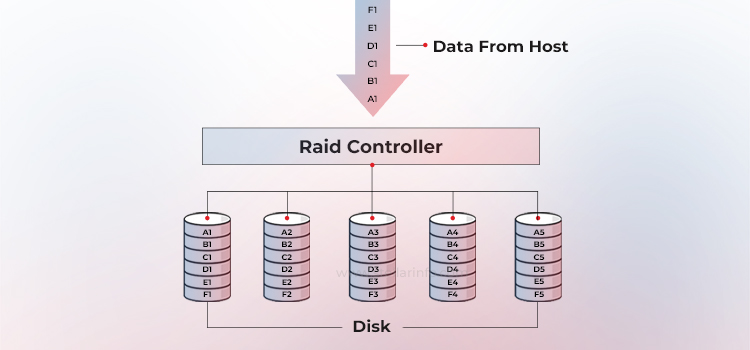
This parity is calculated by the RAID controller using a bitwise XOR operation across all data blocks in a stripe. If one drive fails, the missing block can be rebuilt instantly by XORing the remaining data with the stored parity.
For example, consider three bits: A, B, and C, where A is the parity generated from B and C. Here's how XOR works.
| B | C | A = B ⊕ C |
| 0 | 0 | 0 |
| 0 | 1 | 1 |
| 1 | 0 | 1 |
| 1 | 1 | 0 |
If you know A and one of B or C, you can always recover the third. This is the parity principle RAID uses to rebuild missing data blocks.
Parity information can be stored on a dedicated disk (RAID 4) or distributed across all members (RAID 5). RAID 6 takes it further by adding a second parity block, allowing recovery from two simultaneous failures. The trade-off is a small write penalty: each update modifies both the original data and the parity, requiring extra read–modify–write cycles that reduce performance.
RAID Is a Framework—Each Level Solves a Different Problem
So, the 1988 Berkeley paper did more than coin an acronym—it defined a framework for dialing storage systems up or down along three axes: performance, capacity efficiency, and fault tolerance.
- Pure striping with zero redundancy became RAID 0.
- Add full duplication, and the result is RAID 1, which favors availability over usable terabytes.
- Blend striping with mathematical parity, and you get RAID 5 & 6—configurations that trade some write speed to survive one—or even two—drive losses.
Each configuration is simply a different point in the space the SIGMOD ‘88 paper mapped out.


About The Author

Data Recovery Expert & Content Strategist