In their paper, “A Case for Redundant Arrays of Inexpensive Disks (RAID),” presented at the 1988 SIGMOD Conference, David Patterson, Garth Gibson, and Randy Katz marked one eye-opening baseline: RAID 0. Simply by striping data across cheap PC disks with zero redundancy, they proved it was possible to multiply IO throughput and capacity for pennies—so long as you were willing to risk losing everything if one drive failed.
What Is RAID 0?
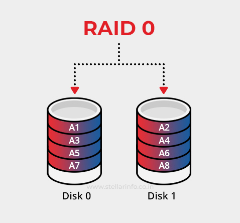
RAID 0—also called striping—is the simplest array organization. It is RAID, but without redundancy. It treats two or more physical drives as a single logical volume and splits every file into equal-sized pieces, or strips. These strips are written to the drives in round-robin order so that all spindles (or channels, in the case of SSDs) work in parallel.
Because no extra copies or parity codes are stored, RAID 0 delivers three headline characteristics:
- Speed: Sequential bandwidth and IOPS (Input/output Operations Per Second) scale up almost linearly with the number of drives.
- Full capacity: You keep 100% of aggregate drive space—no overhead.
- Zero fault tolerance: If any member fails, the stripe set collapses, and you have to seek professional help to recover data from the RAID 0 setup.
This trade-off makes RAID 0 attractive for non-critical workloads—scratch renders, high-speed capture buffers, enthusiast gaming rigs—where raw performance matters more than durability.
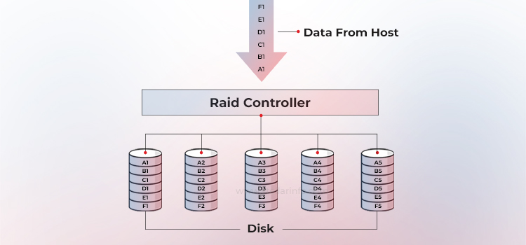
RAID 0 in an array in which data is striped across five disks
How RAID 0, or Striping, Works?
1. Striping logic
The RAID controller (or OS software) chooses a chunk size—say 64 KB. It breaks incoming writes into chunks and assigns them to disks in sequence: chunk 0 to Disk 0, chunk 1 to Disk 1, chunk 2 to Disk 2, and so on, wrapping around when it reaches the last drive.
2. Stripe composition
A set of chunks that share the same logical offset is a stripe. In a four-disk array, the first stripe might hold blocks 0–3 (i.e., one block per disk). Larger chunk sizes—two blocks per disk, for example—yield wider stripes that favor big sequential transfers; smaller chunks improve parallelism on mixed I/O.
3. Read/write behavior
For sequential I/O, the controller issues simultaneous commands to every drive in the stripe, harvesting bandwidth from all spindles at once. Random I/Os are distributed so no single disk becomes a hotspot.
Latency for a single 4 KB read is roughly that of one drive, but aggregate throughput reaches N × S for sequential and N × R for random workloads (where N is drive count, S is sequential read speed in MB/s, and R is random read speed in MB/s).
4. Failure semantics
With no parity or mirrors, the array has no way to reconstruct lost chunks; one dead disk can invalidate every file.
A Working Example of RAID 0
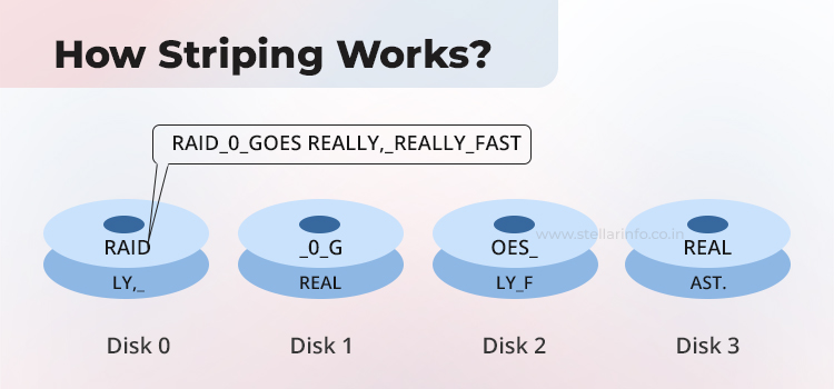
Consider this sentence as a block of data: “RAID_0_goes_really,_really_fast.”
Let’s stripe this six-word phrase across four disks with a chunk size of four characters.
1. Write path
Word 1 (“RAID”) lands on Disk-0.
Word 2 (“_0_g”) on Disk-1, Word 3 (“oes_”) on Disk-2, and Word 4 (“real”) on Disk-3.
The controller then wraps around for the second stripe: “ly,_”→ Disk-0, “real” → Disk-1, “ly_f” → Disk-2, and “ast.” → Disk-3.
2. Read path
A sequential read of the sentence is serviced by four disks at once—each delivers its chunk while the others spin to the next block, giving ~4× the bandwidth of a single drive.
3. Failure scenario
If Disk-2 fails, chunks “oes_” and “ly_f” vanish, corrupting both stripes and making the phrase unreadable. That’s the RAID 0 trade-off: blistering speed, zero tolerance for a failed disk.
RAID 0—Benefits & Limitations
RAID 0 is simply striping without redundancy. It is the base upon which Patterson, Gibson & Katz modelled five different RAID configurations in their 1988 paper, mentioning.
- “75 inexpensive disks potentially have 12 times the I/O bandwidth of the IBM 3380 and the same capacity, with lower power consumption and cost.”
| Characteristic | What it means in practice |
| Performance | Sequential BW ≈ W × (single-drive BW); IOPS scale similarly until the controller’s queue or PCIe lanes saturate. |
| Capacity | Sum of all member drives; no overhead. |
| Reliability | Mean Time To Data Loss (MTTDL) ≈ MTBF / W: every extra drive cuts the mean time to catastrophic loss. A 20-disk RAID 0 can have a ≥ 50 % failure probability within five years, even on enterprise SAS drives. |
| Rebuilds | None—there is nothing to rebuild. Backups or higher-layer replication are mandatory. |
Deployment Scenarios—Where RAID 0 Fits
RAID 0 is suitable in scenarios where raw speed and full capacity matter more than fault tolerance. The table below lists such scenarios with reasons why RAID 0 is successful in these cases.
| Scenario | Why RAID 0 is attractive |
| High-bit-rate video or image production | Massive sequential reads/writes saturate individual disks; striping aggregates bandwidth for smooth 4K/8K timelines and real-time effects. |
| Scratch or render caches in VFX / scientific computing | Datasets are regenerated easily, so losing a volume costs time, not irreplaceable information; parallel stripes cut render I/O bottlenecks. |
| High-speed ingest buffers (lab instruments, camera capture) | Short-term landing zone needs burst writes; after ingest, files move to protected storage. |
| Enthusiast gaming or benchmark rigs | Synthetic tests and load screens show higher transfer rates; risk is acceptable because OS/game images are simple to reinstall. |
| Temporary build or test environments | Continuous-integration pipelines compile artifacts that are re-created each run, favoring compile speed over persistence. |
Deployment Scenarios—Where RAID 0 Should Be Avoided
Despite the allure of speed, RAID 0 is the worst choice for any workload that cannot tolerate data loss or long rebuild times. Consider these use cases.
- Mission-critical databases and transactional systems: A single-disk failure destroys every table; instead, mirrored (RAID 1/10) or parity arrays are the norm.
- Enterprise file shares, archival media, or nearline backup sets: Capacity is large, data is unique, and restore windows must be predictable; instead, RAID 5/6 or erasure coding provide protection with far lower risk.
- Workloads with mixed random I/O that cannot pause for recovery: The performance is marginal, yet recovery from failure requires a full restore from backup.
- Any environment lacking a robust, automated backup strategy: Striping multiplies the chance of volume loss: n drives → n times the failure probability. A two-disk RAID 0 already doubles the risk.
RAID 0 is speed at the price of certainty. Deploy it only when the workload is disposable or protected elsewhere; otherwise, pick a RAID level (or cloud tier) that matches your durability requirements.
RAID 0’s legacy is therefore two-fold: it proved the performance half of the RAID equation, and it reminded every storage architect that speed without durability works only on disposable data.
Beyond RAID 0
RAID 0 proved that striping could deliver massive speed gains—but it also came with a critical flaw: no protection against drive failure. Even a single disk crash would destroy the entire array. For real-world use, especially in enterprise settings where data loss is unacceptable, RAID 0 alone isn’t enough.
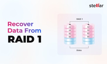
The Berkeley researchers understood this from the beginning. They proposed a full range of RAID levels. Each of these was a usable blend of speed, capacity, and fault tolerance. In the next guide, we’ll explore RAID 1, where data safety takes center stage through mirroring.
Want to learn more about RAID and its alternatives? Here are some related articles worth exploring:
- What Is RAID 1? Characteristics, Benefits, & Limitations
- What Is RAID 5? Design, Advantages, & Drawbacks
- What Is RAID 6? Features, Use Cases, & Data Recovery Options
- RAID Controller Failure: Causes, Symptoms, & Recovery Solutions
- RAID Data Recovery: Call a Specialist Before the Manufacturer’s Helpdesk or DIY


About The Author

Data Recovery Expert & Content Strategist